Acquisition

For each participant, two sets of data were collected: environmental conditions and participants physiological responses. The examples of both data sets, collected through sensors, are given here.

Example data: environmental conditions

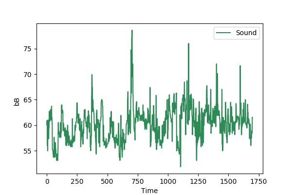
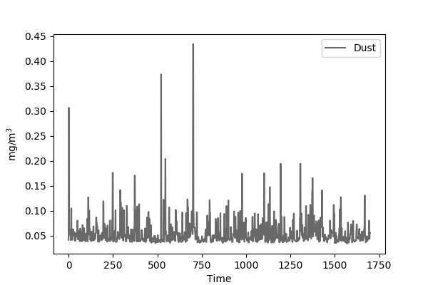
Data collected through Smart Cities Board sensor were sound level and the amount of dust in the environment. An example of data for sound level signal and for dust signal collected during a participants' walk is as follows:

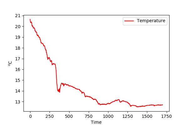
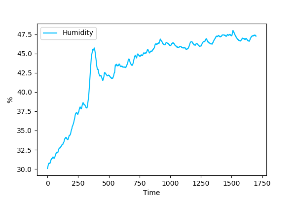
Data collected through HOBO U12 Logger sensor were temperature, humidity, and illuminance in the environment. An example of each of which collected during a participant's walk is shown as follows:

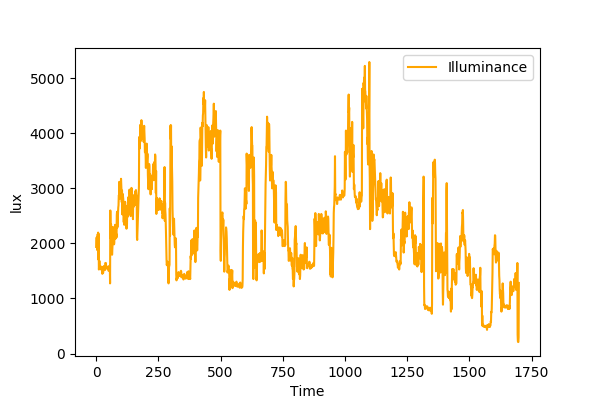Nonetheless, participants’ field-of-view (Isovist) was computed based on the GPS position noted during their walk. Isovist indicates the filed-of-view of a participant that corresponds to a narrow and wider view (space) experienced by a participant during the walk. An example of an Isovist measure is illustrated through an animation as follows:

Example data: Physiological sensor data

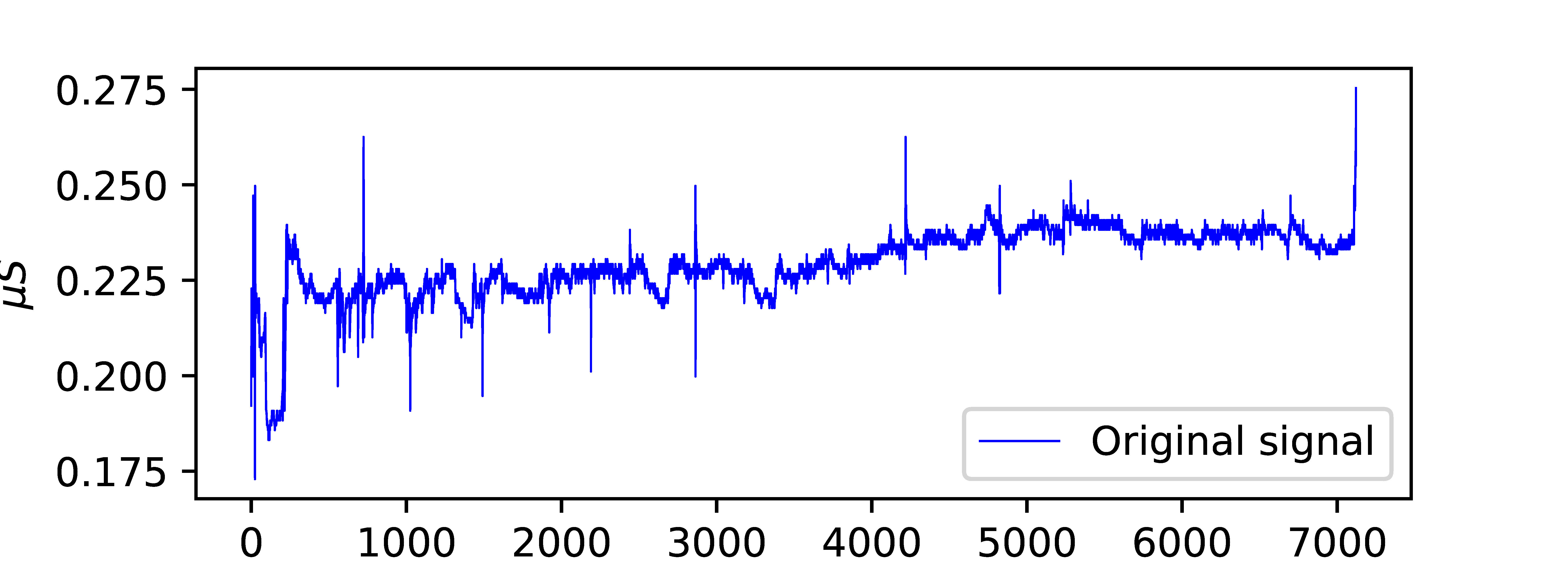
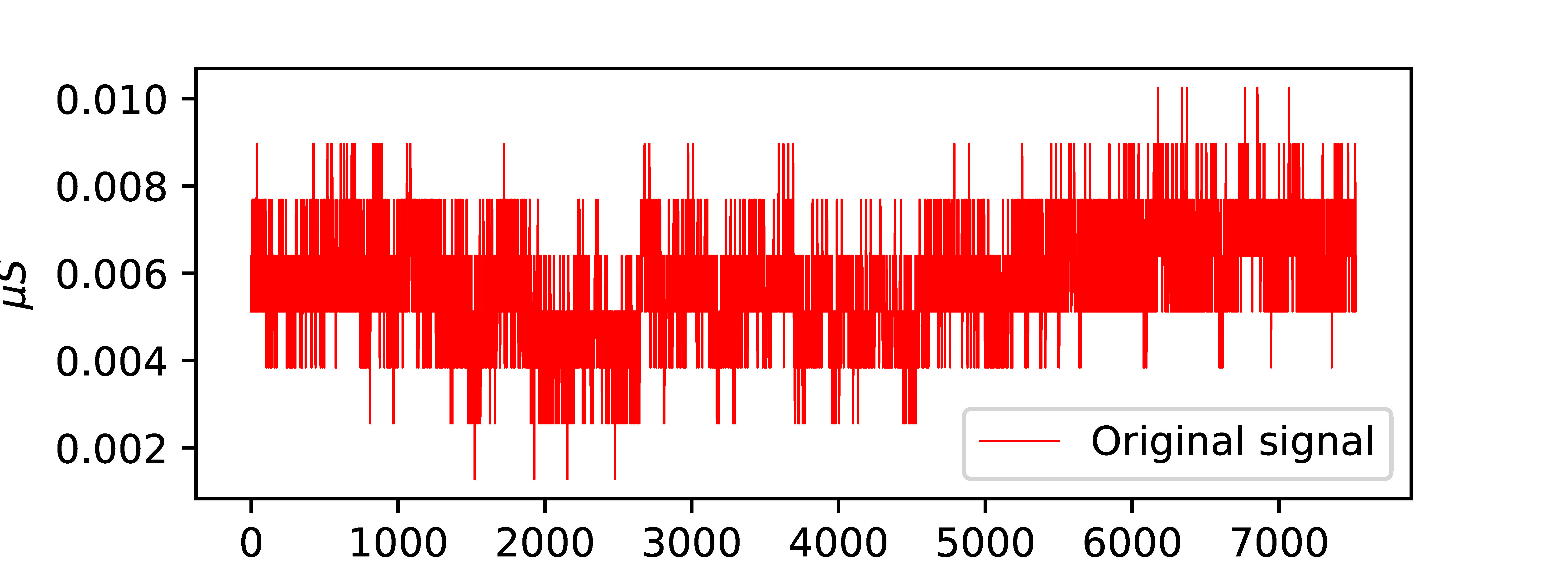
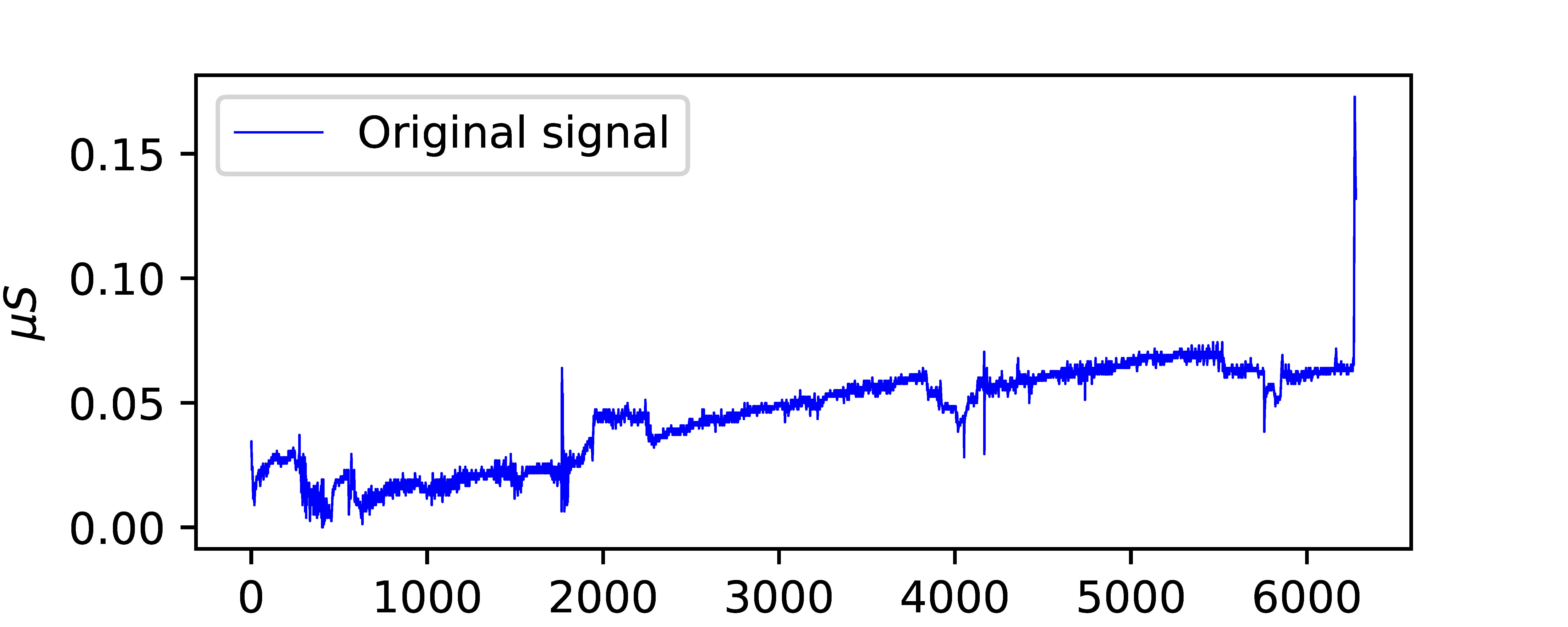
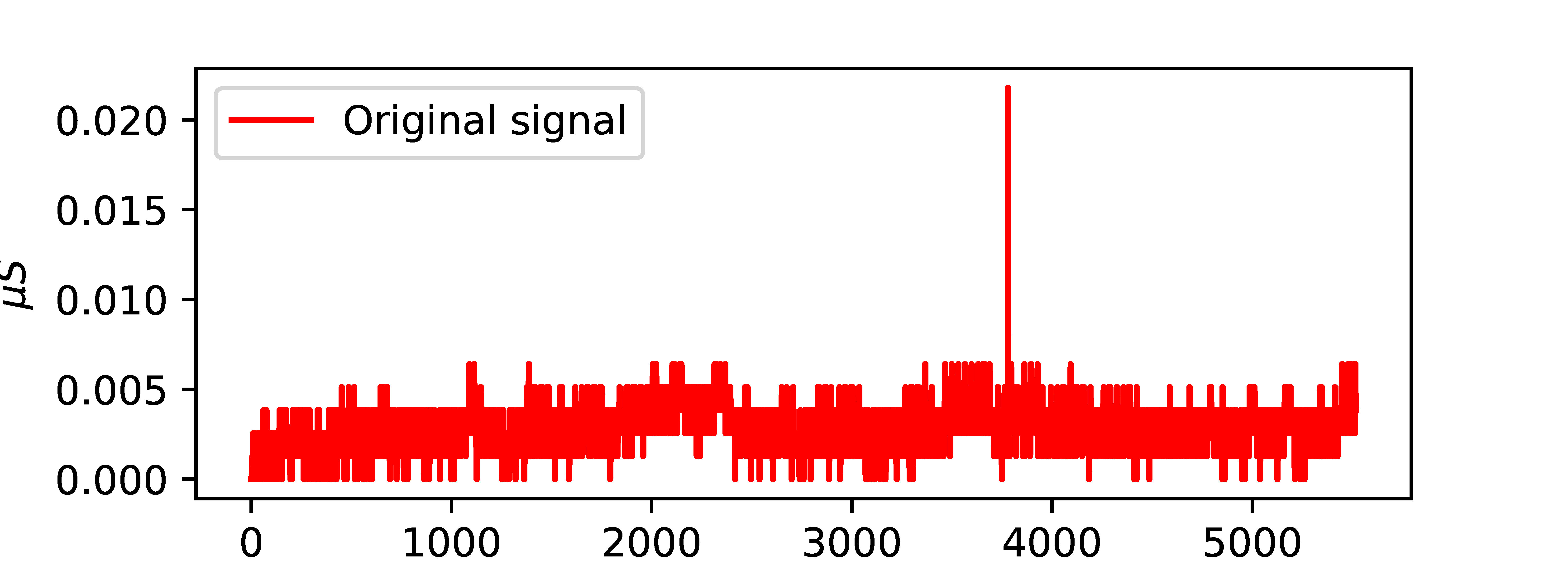
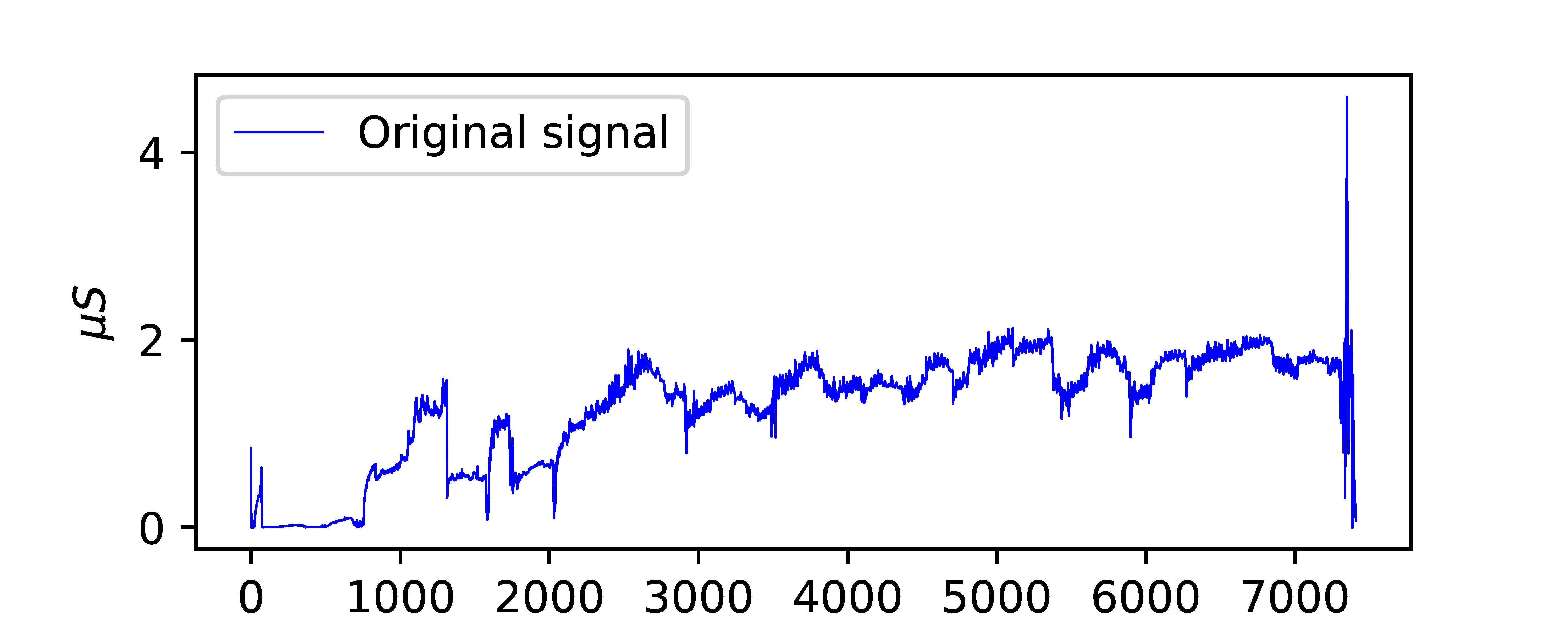
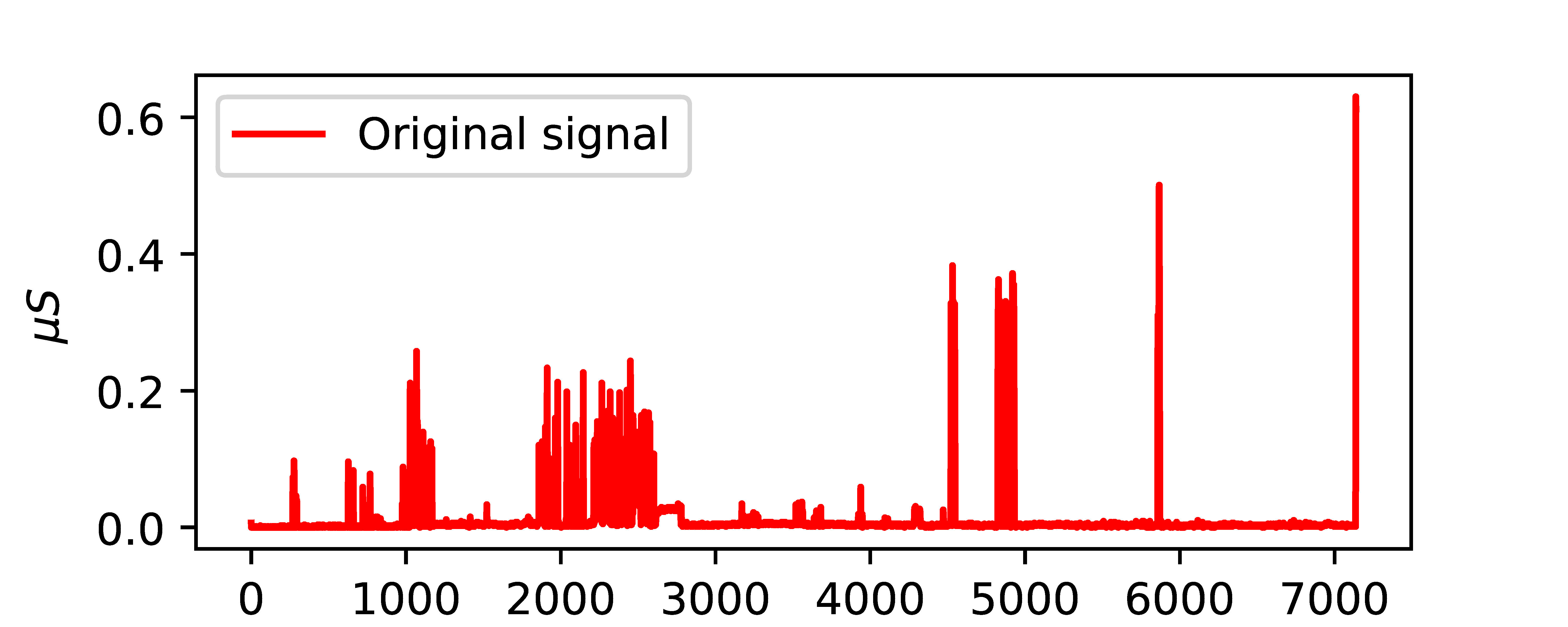
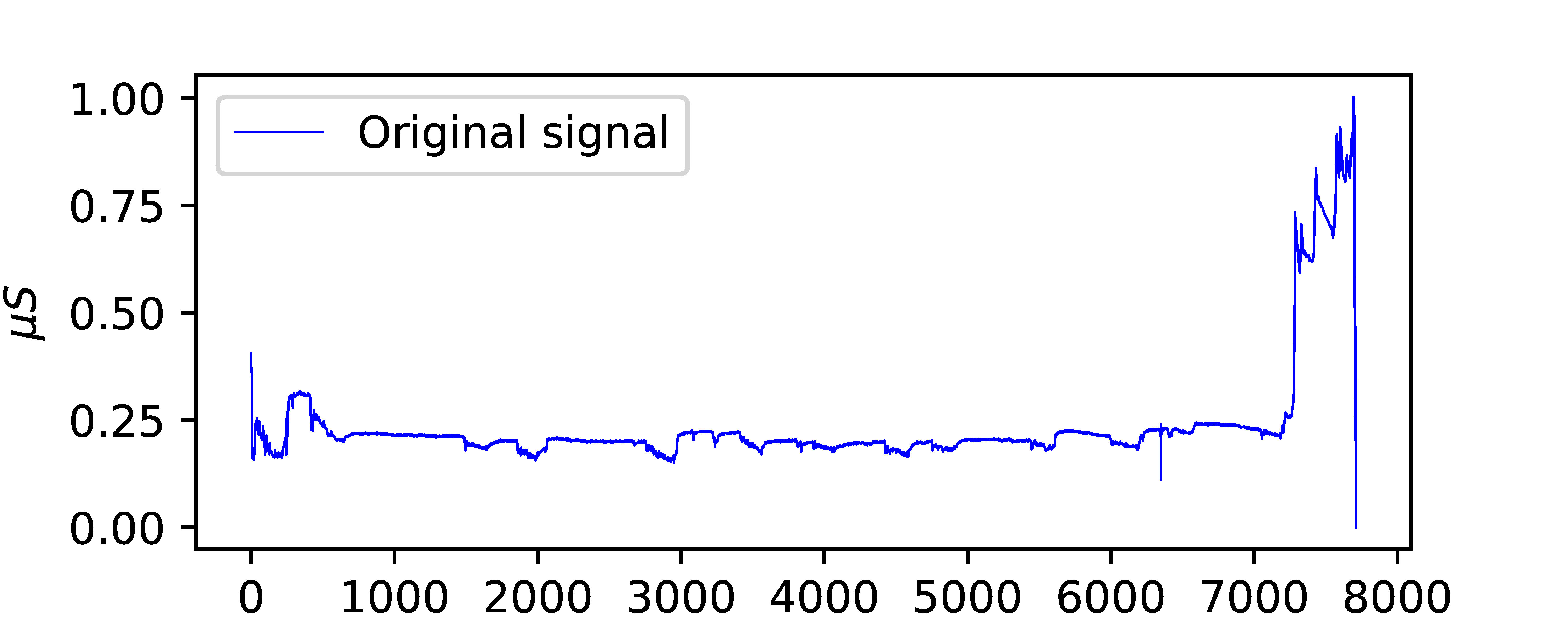
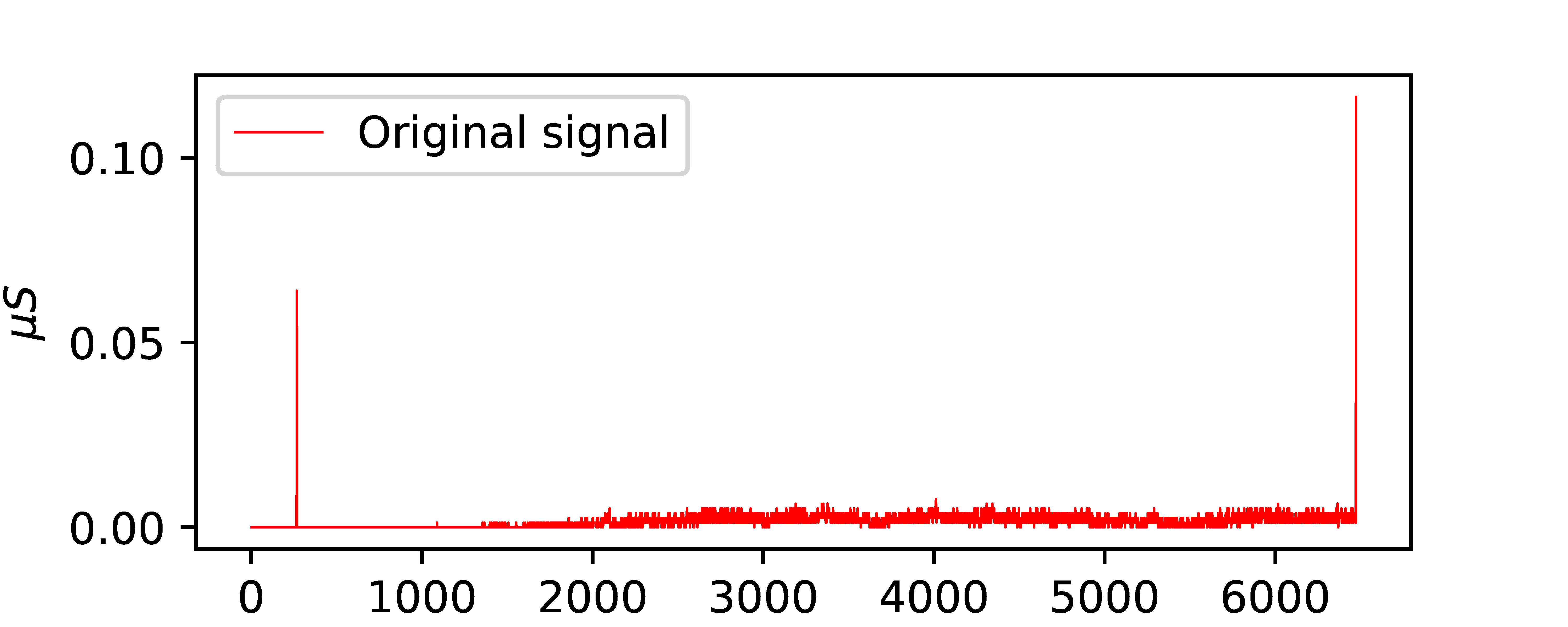
Data collected through the wearable device (Empatica E4) were participants’ physiological responses. It was observed that some of the participants' physiological response data were corrupt and erroneous. Hence, participants’ physiological response data/signal were categorized into two sets: sets of error-free physiological response signals and erroneous physiological response signals. The examples of four types of error-free physiological response signals and four types of erroneous physiological response signals are shown here:

Considered physiological signals	Discarded physiological signals

Depending upon the selection error-free physiological response signals, a total 20 participants data (environmental conditions and physiological responses) were propagated to data preprocessing steps and further data mining steps. In other words, data of 10 participants having erroneous physiological response signals were discarded.

Preprocessing

Data preprocessing involved two steps: smoothing and filtering of physiological response signals and quantification of the environmental conditions signals and physiological response signals.

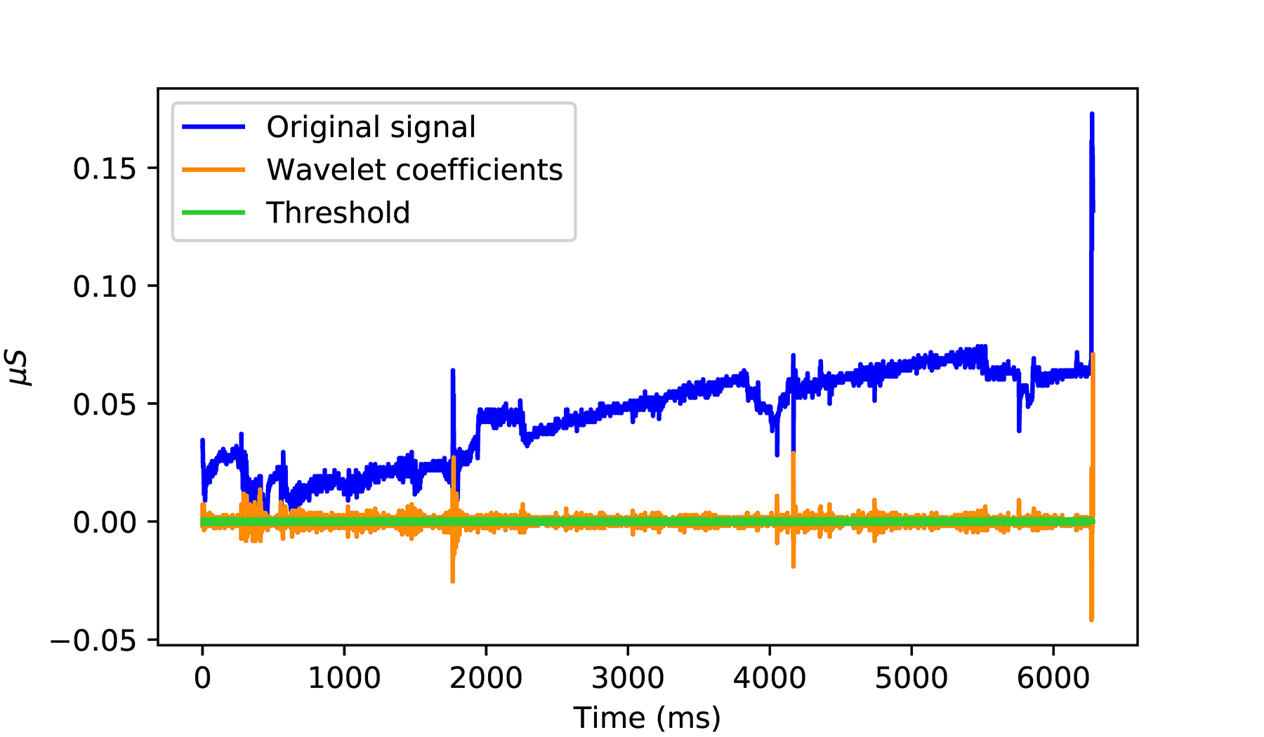
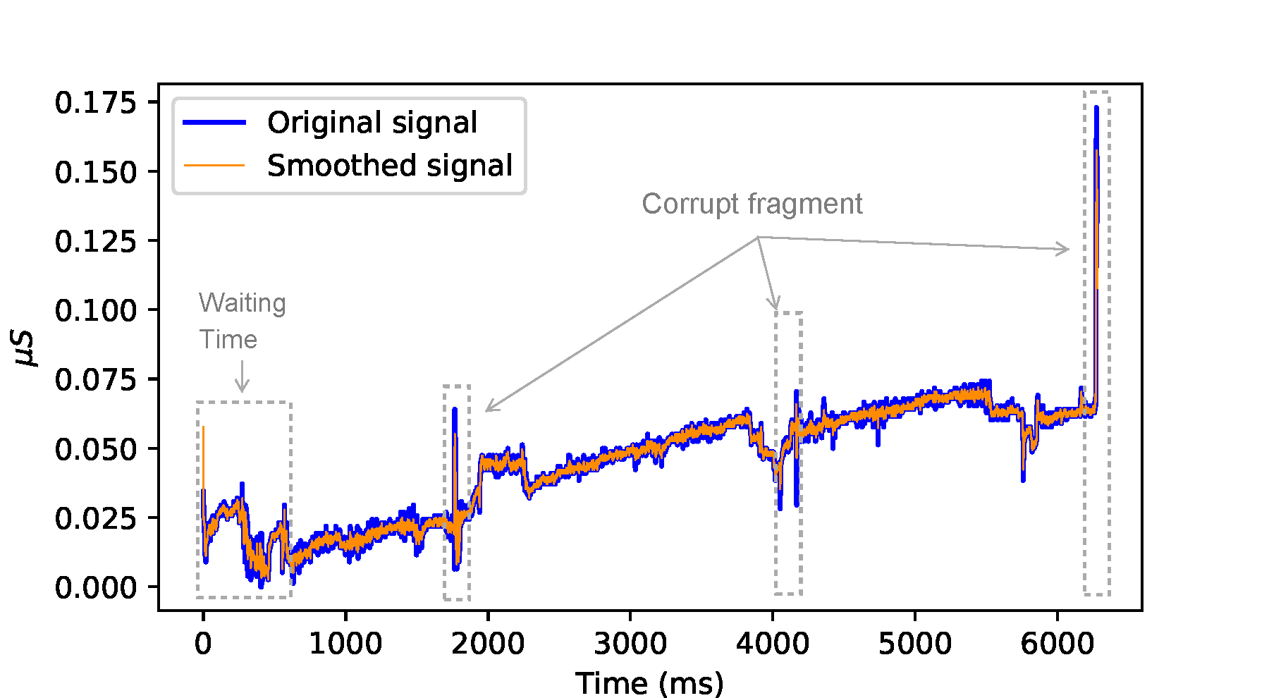
Signal smoothing

Physiological data is known for its sensitivity towards artifacts. Thus, a signal smoothing based on stationary wavelet transform (SWT) and filtering based on information such as an abrupt change in the signal, sensor loss in the signal, and participants waiting time at the start of the walk were performed.

Signal smoothing process	Signal filtering process

Signal quantification

Signals from each sensor were of length A to B, where A and B are UNIX timestamp varied from participant to participants. Each signal was marked start and end of the participants walk. From physiological response data of each participants, only the signal fragment marked start and end is used for data analysis.

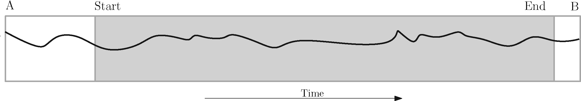
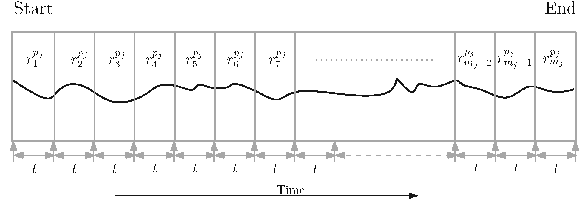
Signals quantification was the major step in the data preprocessing. A conceptual diagram is shown here to illustrate the signals qualification process. A participant walked from start to end point in a city neighborhood. And, for every \(t\) seconds participants' walk, its continuous signals were quantified.

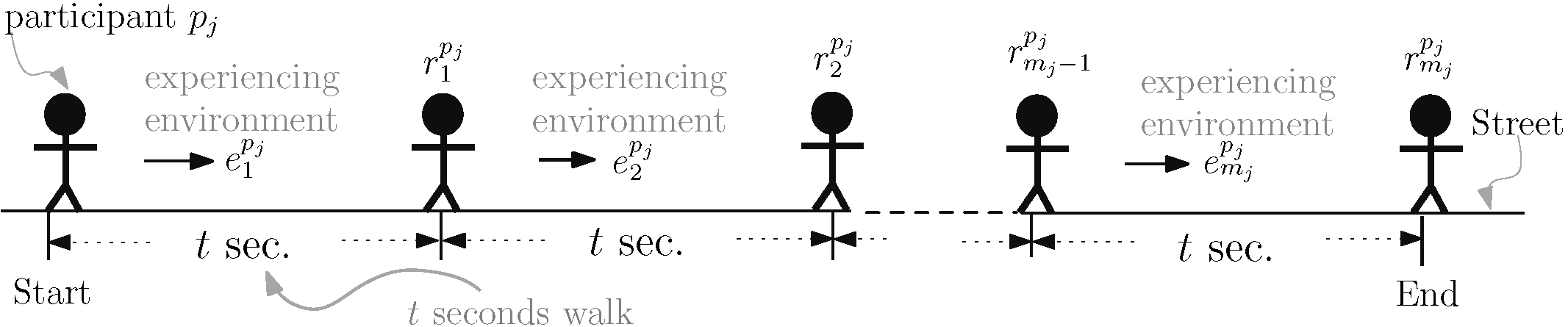
Environmental sensor values \(e_i\) for a \(t\) second window was the average of the signal portion and participants physiological response \(r_i\) for a \(t\) second window was computed using continuous decomposition analysis method described by a tool called Ledalab.

Information Fusion

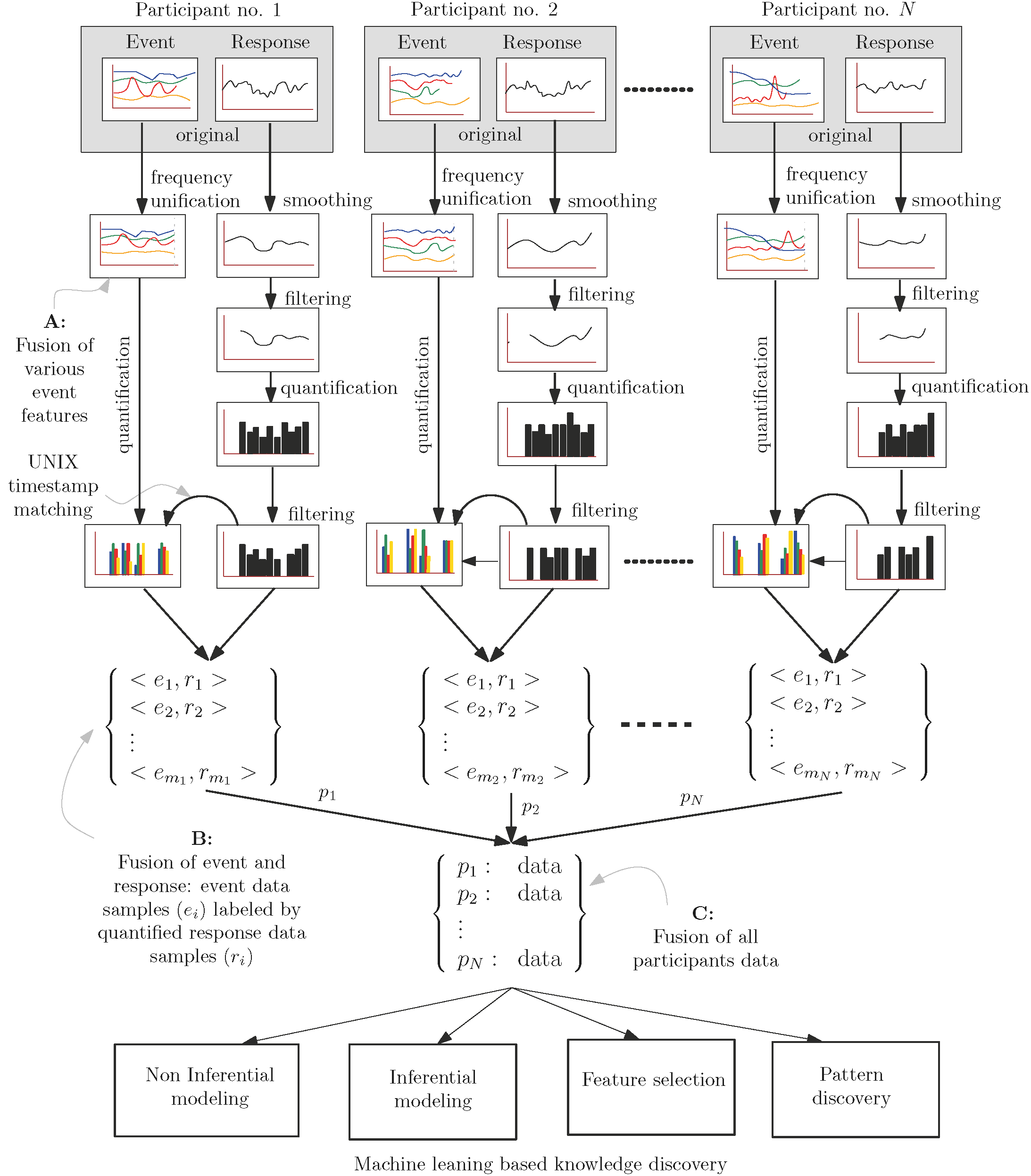
Data in this study are collected from various sensors. Each sensor operated at differing frequencies. Therefore, one-step was to align all sensors signals to a 1 Hz frequency (shown by mark "\(\mathrm{A}\)" in Fig).

Singles from environmental conditions and physiological responses underwent to their respective quantification process. Here, it needs to mention that physiological responses were quantified first and the time window size and UNIX timestamp information were passed to environmental condition signals for their quantification. After quantification of both environmental condition signals and physiological response signals, they were paired as event-response as shown by mark "\(\mathrm{B}\)" in Fig.

Once data of each participant were prepared by pairing event and response, they were further merged together to obtained a compiled data set as shown by mark "\(\mathrm{C}\)" in Fig. The compiled data set thus contained environmental condition (sound, dust, temperature, humidity, illuminance, and Isovist) as the input and participant physiological response as the output.

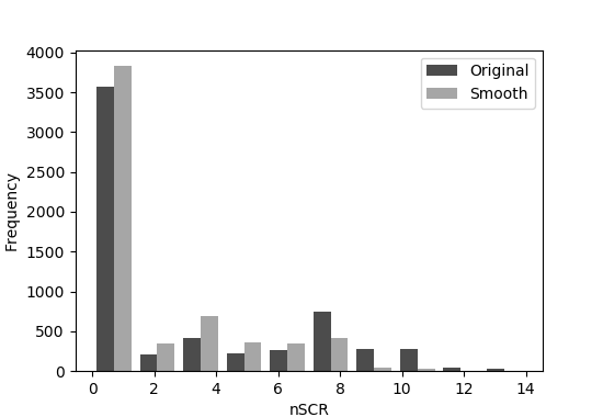
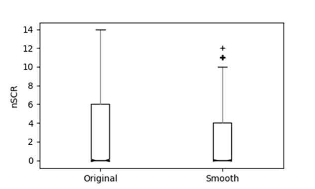
Class label: Quantified physiological response (nSCR) for a time window was within a range of 0 to 14 for an original signal and 0 - 12 for a smooth signal. Hence, to formulate the dataset into a classification problem, nSCR were labeled as 0 when the nSCR value was 0 and 1 when the nSCR value was greater than 0. The distribution and range of nSCR values are illustrated in Fig below.

nCR Histogram	nSCR Box plot

Complied dataset: As per the information fusion stage "\(\mathrm{C}\)" a comprehensive complied dataset was obtained:

Type	Attributes/Features	Definition
Input	Participant ID	Participant identifier used for combined datasets.
	Timestamp	Used to match samples at an instance in time.
	Longitude Latitude	Geographic location associated with each sample, i.e., the location where a time window begins.
	Sound Dust Temperature Relative humidity Brightness/Illuminance	Calculated mean of noise, dust, environment temperature, relative humidity, and illuminance for a time window along the walk.
	Isovist area Isovist perimeter Isovist compactness Isovist occlusivity	Isovist characteristics (Benedikt, 1979) calculated from the field of view for each participant at the corresponding Timestamp, Longitude and Latitude.
Output	Binary/Multiclass/phasic driver	Quantified response of each participants’ individual perception (phasic nSCR) (Section 3.2.3).

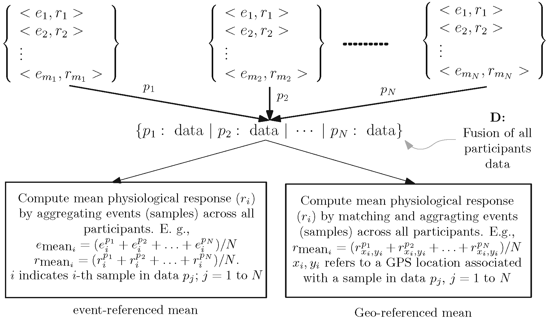
Correlation and Geo-reference analysis framework: To compute the correlation between environmental conditions experienced across all participants and the physiological arousal across all participants, participants event-referenced mean were computed.

Similarly, to investigate average physiological responses across all participants associated with a geographical location, geo-referenced mean were computed.

The framework for fusing information to compute event-referenced and geo-referenced means was designed as per the following:

Downloads

Research paper:

Ojha VK, Griego D, Kuliga S, Bielik M, Buš P, Schaeben C, Treyer L, Standfest M, Schneider S, König R, Donath D, Schmitt G (2018) Machine learning approaches to understand the influence of urban environments on human’s physiological response, Information Sciences, Elsevier (pdf).

Data

Download raw and processed data directly. The data are in ZIP folder. Following are the subprojects of ESUM:

ESUM SNF Project data

Bus Stop study data (Commuting Experience data)

Virtual Reality Experiment data

Codes

Download the codes from the GitHub. The codes are mainly for data preprocessing and visualization. The codes are mostly written in python. Following are the subprojects of ESUM:

ESUM SNF project data processing codes

ESUM+ commuting experience (Bus Stop study) data processing codes

360 Virtual Reality data processing codes

Block Geometry data processing codes

ESUM: Data Visualization Tool

Presentations

ESUM complete picture (pdf)
Machine learning and pattern analysis for ESUM (pdf)
MAPS: Visual representation of results (pdf)
Talk delivered in ITA, ETH Zurich, Switzerland (pdf)
Falling Wall competition Paris, France (presentation won 3rd place): (pdf)
Information Visualization: People's commuting experience in cities (pdf)

Dissertation

Silvennoinen, H. (2018) Non-Spatial and Spatial Statistics for Analysing Human's Perception of the Built Environment, ETH Zurich, Switzerland (pdf, code)

Stolbovoy, V. (2018) Convolutional Neural Network and Visual Feature Extraction for Evaluation of the Urban Environment, ETH Zurich, Switzerland (pdf, code)

Schaeben, C. (2017) People's Perception of Urban and Architectural Features, ETH Zurich, Switzerland (pdf)